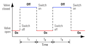
A diagram of the switching action
of the thermostat would look like the graph shown.
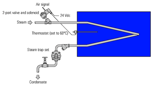
The temperature of the tank contents will fall to
59°C before the valve opens and will rise to 61°C
before the valve closes.
It will take time for the steam in the coil to affect 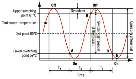 the temperature of the water in the tank and the
water in the tank will rise abovethe 61°C upper limit
and fall below the 59°C lower limit.
At point A (59°C) the thermostat switches on,
and opens the valve. It takes time for the
transfer of heat from the coil to affect the
water temperature, as shown by the graph.
At point B (61°C) the thermostat switches off
and shuts the valve. However the coil is still
full of steam, which continues to condense
and give up its heat. Hence the water temperature continues to rise above the upper switching temperature,
and 'overshoots' at C, before eventually falling.
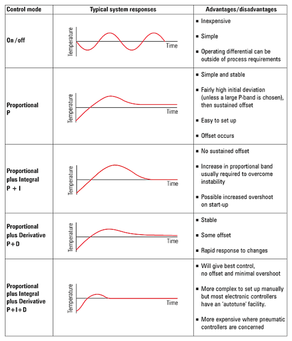
The main advantages of on/off control are simplicity and low cost.
This is why it is frequently found on domestic applications such
as oven toasters and AC units. Its major disadvantage is that
the operating differential might fall outside the control tolerance
required by the process. For example, on a distillation column,
where product separation is achieved through precise
temperature control, on/off control would be unsuitable.
If accurate temperature control is required,
the option is Proportional control.
Proportional control
Proportional control is often called modulating control.
It means that the valve is capable of changing
the amount of valve opening. It does not just move
to either fully open or fully closed, as with on-off control.
The three basic control actions are:
Proportional (P)
Integral (I)
Derivative (D)
It is also necessary to consider these in combination such as P + I, P + D, P + I + D.
Although it is possible to combine the different actions, and all help to produce the
required response, it is important to remember that both the integral and derivative
actions are corrective functions of the basic proportional control action.
Proportional control
This is the most basic of the control actions and is usually referred to as 'P'.
The principle aim of proportional control is to control the process as the conditions change.
The unit of ‘P’ is the proportional band expressed in %.
The larger the proportional band, the more stable the control,
but the greater the offset.
The narrower the proportional band, the less stable the process,
but the smaller the offset.
The aim, therefore, should be to set the smallest proportional band
that will always keep the process stable with the minimum offset.
Gain
The term 'gain' is often used with controllers and
is simply the reciprocal of proportional band.
The larger the controller gain, the more the
controller output will change for a given error.
For instance for a gain of 1, an error of 10% of scale
will change the controller output by 10% of scale,
for a gain of 5, an error of 10% will change the controller
output by 50% of scale, whilst for a gain of 10,
an error of 10% will change the output by 100% of scale.
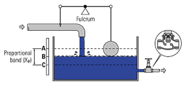
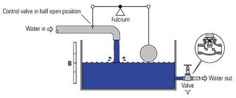
The system is in balance (the flowrate of water entering and leaving the tank is the same); under control,
in a stable condition (the level is not varying)
and at precisely the desired water level (B );
giving the required outflow. System Balanced Water In = Water Out
One recognized symbol for Proportional Band is Xp. The control valve is moved in proportion to the error in the water level
(or the temperature deviation, in the case of a temperature control)
from the set point.
The set point can only be maintained for one specific load condition.
Whilst stable control will be achieved between points A and C,
any load causing a difference in level to that of B will always provide an offset.
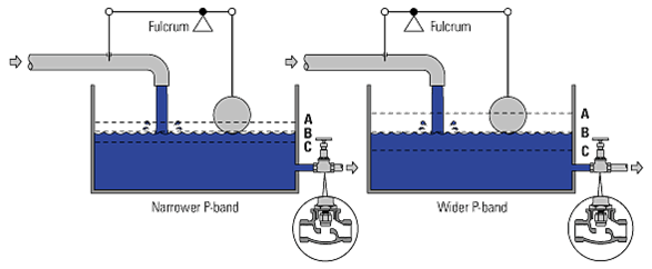
By altering the fulcrum position, the system Proportional Band changes.
Nearer the float gives a narrower P-band, whilst nearer the valve gives a wider P-band.
Different fulcrum positions require different changes in water level to move the valve from fully open to fully closed. In both cases, It can be seen that level B represents the 50% load level, A represents the 0% load level, and C represents the 100% load level.
Demonstrating the relationship between P-band and offset
Proportional band is the level (or perhaps temperature or pressure etc.)
change required to move the valve from open to fully closed.
This is convenient for mechanical systems, but a more general (and more correct)
definition of proportional band is the percentage change in
measured valuerequired to give a 100% change in output.
It is therefore usually expressed in percentage terms rather than
in engineering units such as degrees centigrade.
For electrical and pneumatic controllers, the
set value is at the middle of the proportional band.
The effect of changing the P-band for an electrical or pneumatic system can be described with a slightly different example, by using a temperature control.
The space temperature of a building is controlled by a water
(radiator type) heating system using a proportional action
control by a valve driven with an electrical actuator,
and an electronic controller and room temperature sensor.
The control selected has a proportional band (P-band or Xp)
of 6% of the controller input span of 0° - 100°C,
and the desired internal space temperature is 18°C.
Under certain load conditions, the valve is 50% open
and the required internal temperature is correct at 18°C
The room temperature is currently 18°C, and the valve is 50% open.
The proportional band is set at 6% of 100°C = 6°C,
which gives 3°C either side of the 18°C set point.
A fall in outside temperature occurs,. consequently,
the internal temperature will decrease.
This is detected by the room temperature sensor,
which signals the valve to move to a more open position allowing
hotter water to pass through the room radiators.
The valve is instructed to open by an amount
proportional to the drop in room temperature.
In simplistic terms, if the room temperature falls by 1°C,
the valve may open by 10%; if the room temperature falls by 2°C,
the valve will open by 20%.
In due course, the outside temperature stabilises
and the inside temperature stops falling.
In order to provide the additional heat required for the lower
outside temperature, the valve will stabilise in a more open position;
but the actual inside temperature will be slightly lower than 18°C.
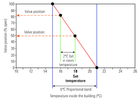
Room temperature and valve relationship - 6°C proportional band
As an example, the room temperature falls to 16°C.
From the chart it can be seen that the new valve opening will be approximately 83%.
With proportional control, if the load changes, so too will the offset:
A load of less than 50% will cause the room temperature to be above the set value.
A load of more than 50% will cause the room temperature to be below the set value.
The deviation between the set temperature on the controller (the set point)
and the actual room temperature is called the 'proportional offset‘.
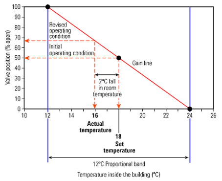
Increasing the P-band - For example, if the previous application had
been programmed with a 12% proportional band equivalent to 12°C,
the results can be seen the illustration.
The wider P-band results in a less steep 'gain' line.
For the same change in room temperature the valve movement will be smaller.
In this instance, the 2°C fall in room temperature would
give a valve opening of about 68% from the chart.
Room temperature and valve relationship - 12°C Proportional band
Reducing the P-band - Conversely, if the P-band is reduced,
the valve movement per temperature increment is increased.
However, reducing the P- band to zero gives an on/off control.
The ideal P- band is as narrow as possible without causing
oscillation in the actual room temperature.
As a reminder:
A wide proportional band (small gain) will provide a less
sensitive response, but a greater stability.
A narrow proportional band (large gain) will provide a more sensitive
response, but there is a practical limit to how narrow the Xp can be set.
Too narrow a proportional band (too much gain) will result
in oscillation and unstable control.
Reverse or direct acting control signal
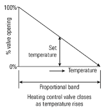
A closer look at the figures used so far to describe the effect of
proportional control shows that the output is assumed to be reverse acting.
In other words, a rise in process temperature causes the
control signal to fall and the valve to close.
This is usually the situation on heating controls.
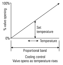
This configuration would not
work on a cooling control; here the valve
must open with a rise in temperature.
This is termed a direct acting control signal
Reverse acting signal Direct acting signal Gain line offset or proportional effect
From the explanation of proportional control, it should be clear that there is a control
offset or a deviation of the actual value from the set value whenever the load varies from 50%.
To further illustrate this, consider a 12°C P- band, where an offset of 2°C was expected.
If the offset cannot be tolerated by the application, then it must be eliminated.
This could be achieved by relocating (or resetting) the set point to a higher value.
This provides the same valve opening after manual reset but at a room temperature
of 18°C not 16°C
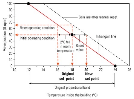 .
. Gain line offset
Manual reset
The offset can be removed either manually or automatically.
The effect of manual reset can be seen in the chart, and the value
is adjusted manually by applying an offset to the set point of 2°C.
It should be clear from chart and the above text that the effect
is the same as increasing the set value by 2°C.
The same valve opening of 66.7% now coincides with the room temperature at 18°C.
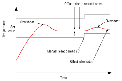
Effect of manual resetIntegral control - automatic reset
'Manual reset' is usually unsatisfactory in process plant where each load change will
require a reset action. It is also quite common for an operator to be
confused by the differences between:
Set value - What is on the dial.
Actual value - What the process value is.
Required value - The perfect process condition.
Such problems are overcome by the reset
action being contained within the mechanism of an automatic controller.
Such a controller is primarily a proportional controller. It then has a reset function
added, which is called 'integral action'. Automatic reset uses an electronic
or pneumatic integration routine to perform the reset function.
The most commonly used term for automatic reset is integral action, which is given the letter I.
The function of integral action is to eliminate offset by continuously and automatically
modifying the controller output in accordance with the control deviation integrated over time.
The Integral Action Time (IAT) is the time taken for the controller output to change
due to the integral action to equal the output change due to the proportional action.
Integral action gives a steadily increasing corrective action as long as an error
continues to exist. Such corrective action will increase with time and must therefore,
at some time, be sufficient to eliminate the steady state error altogether,
providing sufficient time elapses before another change occurs.
The integral action on a controller is often restricted to within the proportional band.
A typical P + I response for a step change in load.
Integral action is also called reset.
If it is too short, over-reaction and instability will result.
If it is too long, reset action will be very slow to take effect.
IAT is represented in time units. On some controllers the adjustable parameter
for the integral action is termed 'repeats per minute', which is the number of
times per minute that the integral action output changes by the proportional output change.
Repeats per minute = 1/(IAT in minutes) IAT = Infinity - Means no integral action
IAT = 0 - Means infinite integral action
It is important to check the controller manual to see how integral action is designated.
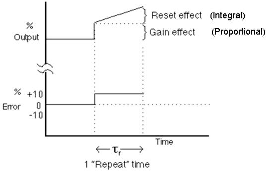
The input to the controller is changed by a small amount. The output will move suddenly due to the gain.
The output will continue to change at a constant rate.
The repeat time, or reset time, is the time it takes for the reset
effect to repeat (or move the output the same amount as) the gain effect.
Derivative control or rate action
A Derivative action (referred to by the letter D) measures and responds
to the rate of change of process signal, and adjusts the output
of the controller to minimise overshoot.
If applied properly on systems with time lags, derivative action will minimise
the deviation from the set point when there is a change in the process condition.
It is interesting to note that derivative action will only
apply itself when there is a change in process signal.
If the value is steady, whatever the offset, then derivative action does not occur.
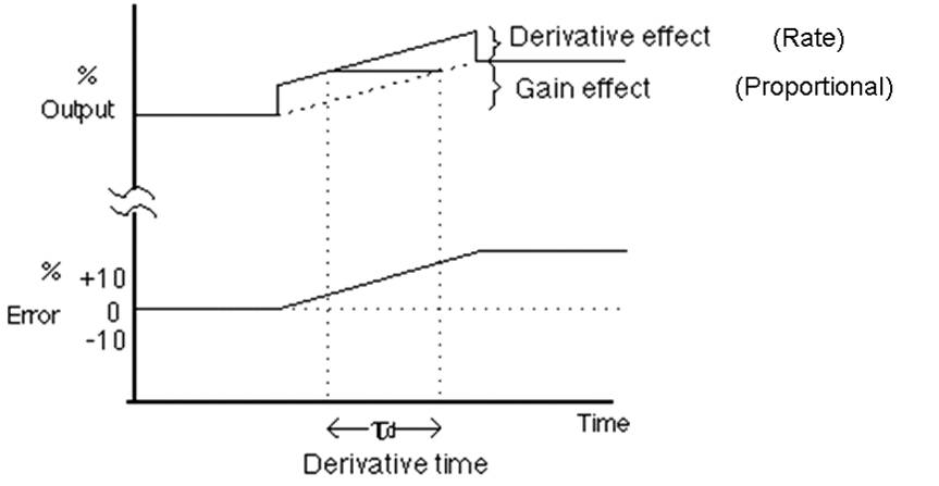
Note that when the ramp is started, with no derivative (dashed line) the output ramps up due to the change in input and the gain.
Using derivative (solid line) the output jumps up, rises in a ramp, then jumps down.
The difference in time between the solid line and the dashed line
represents the amount of derivative, in units of time (usually minutes).
One useful function of the derivative function is that overshoot can be
minimised especially on fast changes in load.
However, derivative action is not easy to apply properly;
if not enough is used, little benefit is achieved,
and applying too much can cause more problems than it solves.
D action is again adjustable within the controller,
and referred to as TD in time units:
T D = 0 - Means no D action.
T D = Infinity - Means infinite D action.
P + D controllers can be obtained, but with proportional offset.
It is worth remembering that the main disadvantage with a P control is
the presence of offset. To overcome and remove offset, 'I' action is introduced.
The frequent existence of time lags in the control loop explains the need
for the third action D. The result is a P + I + D controller which,
if properly tuned, can in most processes give a rapid
and stable response, with no offset and without overshoot.
PID controllers
P and I and D are referred to as 'terms' and thus a
P + I + D controller is often referred to as a three term controller
Hunting
Often referred to as instability, cycling or oscillation.
Hunting produces a continuously changing deviation from the normal operating point.
This can be caused by:
The proportional band being too narrow.
The integral time being too short. The derivative time being too long. A combination of these.
Long time constants or dead times in the control system or the process itself
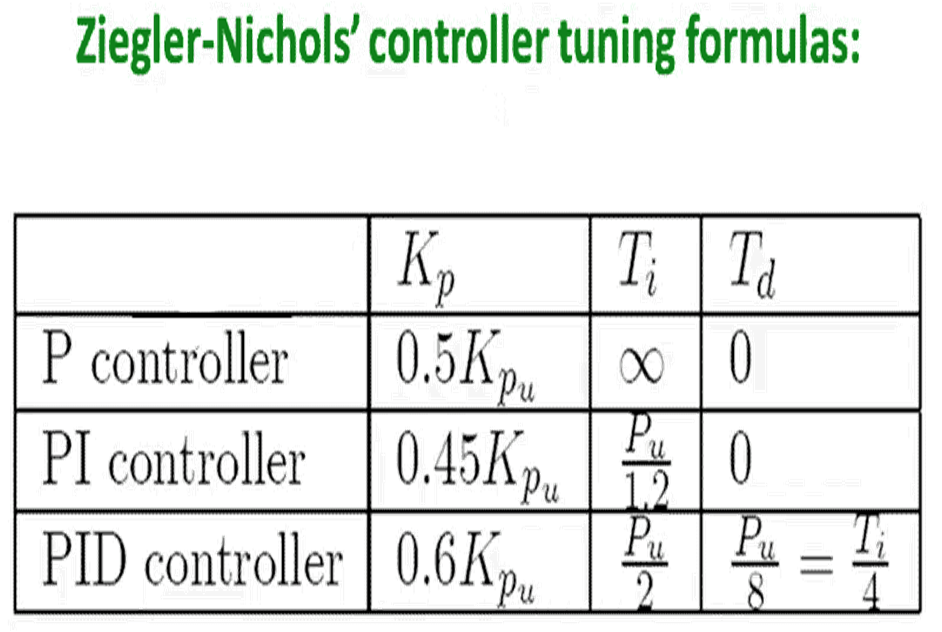
Controller Tuning Methods
Initial Tuning
Initial controller tuning may be used during control system design.
The values are conservative and will result normally in sluggish response.
Once the plant is online, the tuning should be refined based
on the observed process dynamics and gain.
Feedback Control
Advantages
1. Corrective action occurs as soon as the controlled variable deviates
from the set point, regardless of the source and type of disturbance.
2. Feedback control requires minimal knowledge about the process to be controlled;
in particular, a mathematical model of the process is not required,
although it can be very useful for control system design.
3. The ubiquitous PID controller is both versatile and robust.
If process conditions change, retuning the controller usually produces satisfactory control.
Disadvantages
1. Corrective action is taken only until after a deviation in the controlled variable occurs.
Thus, perfect control, wherethe controlled variable does not deviate from the set point
during disturbance or set-point changes, is theoretically impossible.
2. Does not provide predictive control action to compensate for the effects
of known or measurable disturbances.
3. It may not be satisfactory for processes with large time constants and/or long time delays.
If large and frequent disturbances occur, the process may operate continuously
in a transient state and never attain the desired steady state.
4. In some situations, the controlled variable cannot be measured on-line,
and, consequently, feedback control is not feasible.
Feedforward Control
The basic concept of feedforward control is to measure important disturbance
variables and take corrective action before they upset the process.
Feedforward control has several disadvantages:
1.The disturbance variables must be measured on-line. In many applications, this is not feasible.
2. To make effective use of feedforward control, at least a crude process
model should be available. In particular, we need to know how the
controlled variable responds to changes in both the disturbance and manipulated variables.
The quality of feedforward control depends on the accuracy of the process model.
3. Ideal feedforward controllers that are theoretically capable
of achieving perfect control may not be physically realizable.
Fortunately, practical approximations of these ideal controllers often provide very effective control.
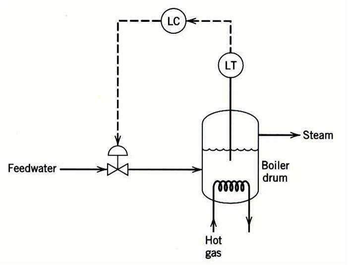
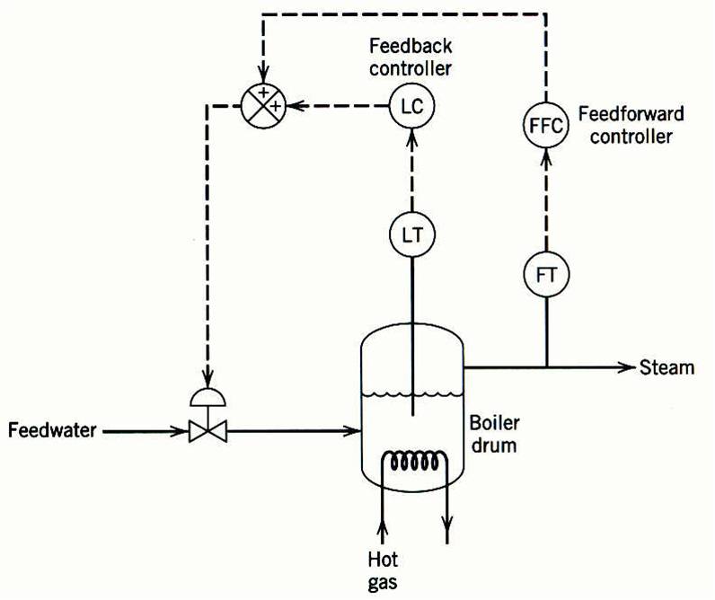
The feedback control of the liquid level in a boiler drum.
A boiler drum with a conventional feedback control system is shown .
The level of the boiling liquid is measured and used to adjust the feedwater flow rate.
This control system tends to be quite sensitive to rapid changes in the disturbance variable,
steam flow rate, as a result of the small liquid capacity of the boiler drum.
Rapid disturbance changes can occur as a result of steam demands
made by downstream processing units.
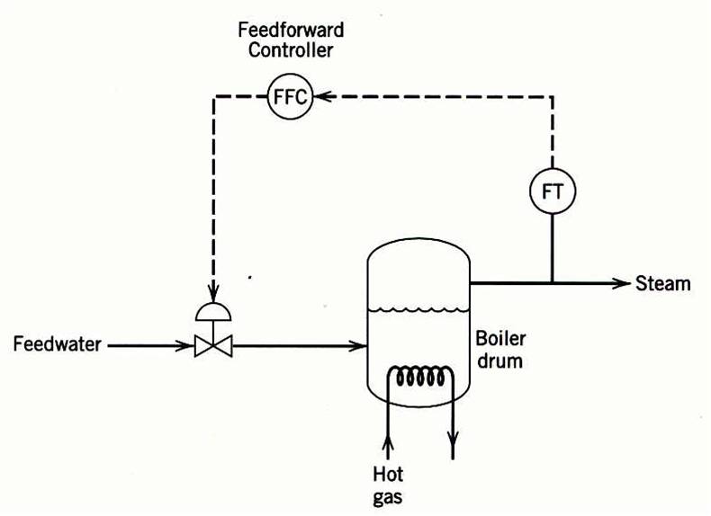
The feedforward control can provide better control of the liquid level.
Here the steam flow rate is measured, and the feedforward
controller adjusts the feedwater flow rate.
The feedforward control of the liquid level in a boilerdrum.
The feedfoward-feedback control of the boiler drum level.
In practical applications, feedforward control is normally used in combination with feedback control.
Feedforward control is used to reduce the effects of measurable disturbances,
while feedback trim compensates for inaccuracies in the process model,
measurement error, and unmeasured disturbances.
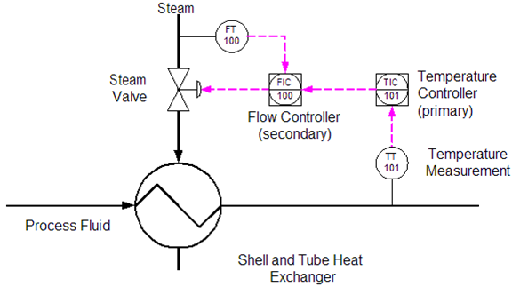
Cascade Control
Cascade Control uses the output of the primary controller to manipulate
the setpoint of the secondary controller as if it were the final control element.
Reasons for cascade control:
1. Allow faster secondary controller to handle disturbances in the secondary loop.
2. Allow secondary controller to handle non- linear valve and other final control element problems.
3. Allow operator to directly control secondary loop during certain modes of operation (such as startup)
email: calmansys@yahoo.com

 The more complex or dangerous the plant or process,
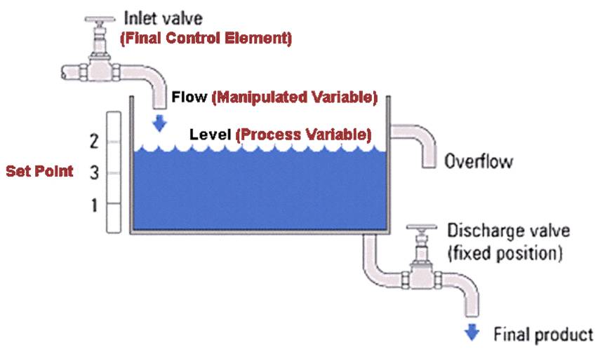 The water level is not too low;